Mathematical formulations of measurements

Noch nich ibersetzt

Die Seide is noch nich ibersetzt worn. Se guggen de englsche Originalversion.

The lesson begins with two equivalent mathematical descriptions of measurements:

1. General measurements can be described by collections of matrices, one for each measurement outcome, in a way that generalizes the description of projective measurements.
2. General measurements can be described as channels whose outputs are always classical states (represented by diagonal density matrices).

We'll restrict our attention to measurements having finitely many possible outcomes. Although it is possible to define measurements with infinitely many possible outcomes, they're much less typically encountered in the context of computation and information processing, and they also require some additional mathematics (namely measure theory) to be properly formalized.

Our initial focus will be on so-called destructive measurements, where the output of the measurement is a classical measurement outcome alone — with no specification of the post-measurement quantum state of whatever system was measured. Intuitively speaking, we can imagine that such a measurement destroys the quantum system itself, or that the system is immediately discarded once the measurement is made. Later in the lesson we'll broaden our view and consider non-destructive measurements, where there's both a classical measurement outcome and a post-measurement quantum state of the measured system.

Measurements as collections of matrices

Suppose $\mathsf{X}$ is a system that is to be measured, and assume for simplicity that the classical state set of $\mathsf{X}$ is $\{0,\ldots, n-1\}$ for some positive integer $n,$ so that density matrices representing quantum states of $\mathsf{X}$ are $n\times n$ matrices. We won't actually have much need to refer to the classical states of $\mathsf{X},$ but it will be convenient to refer to $n,$ the number of classical states of $\mathsf{X}.$ We'll also assume that the possible outcomes of the measurement are the integers $0,\ldots,m-1$ for some positive integer $m.$

Note that we're just using these names to keep things simple; it's straightforward to generalize everything that follows to other finite sets of classical states and measurement outcomes, renaming them as desired.

Projective measurements

Recall that a projective measurement is described by a collection of projection matrices that sum to the identity matrix. In symbols,

$$\{\Pi_0,\ldots,\Pi_{m-1}\}$$

describes a projective measurement of $\mathsf{X}$ if each $\Pi_a$ is an $n\times n$ projection matrix and the following condition is met.

$$\Pi_0 + \cdots + \Pi_{m-1} = \mathbb{I}_{\mathsf{X}}$$

When such a measurement is performed on a system $\mathsf{X}$ while it's in a state described by some quantum state vector $\vert\psi\rangle,$ each outcome $a$ is obtained with probability equal to $\|\Pi_a\vert\psi\rangle\|^2.$ We also have that the post-measurement state of $\mathsf{X}$ is obtained by normalizing the vector $\Pi_a\vert\psi\rangle,$ but we're ignoring the post-measurement state for now.

If the state of $\mathsf{X}$ is described by a density matrix $\rho$ rather than a quantum state vector $\vert\psi\rangle,$ then we can alternatively express the probability to obtain the outcome $a$ as $\operatorname{Tr}(\Pi_a \rho).$

If $\rho = \vert \psi\rangle\langle\psi\vert$ is a pure state, then the two expressions are equal:

$$\operatorname{Tr}(\Pi_a \rho) = \operatorname{Tr}(\Pi_a \vert \psi\rangle\langle\psi \vert) = \langle \psi \vert \Pi_a \vert \psi \rangle = \langle \psi \vert \Pi_a \Pi_a \vert \psi \rangle = \|\Pi_a\vert\psi\rangle\|^2.$$

Here we're using the cyclic property of the trace for the second equality, and for the third equality we're using the fact that each $\Pi_a$ is a projection matrix, and therefore satisfies $\Pi_a^2 = \Pi_a.$

In general, if $\rho$ is a convex combination

$$\rho = \sum_{k = 0}^{N-1} p_k \vert \psi_k\rangle\langle \psi_k \vert$$

of pure states, then the expression $\operatorname{Tr}(\Pi_a \rho)$ coincides with the average probability for the outcome $a,$ owing to the fact that this expression is linear in $\rho.$

$$\operatorname{Tr}(\Pi_a \rho) = \sum_{k = 0}^{N-1} p_k \operatorname{Tr}(\Pi_a \vert \psi_k\rangle\langle\psi_k\vert) = \sum_{k = 0}^{N-1} p_k \|\Pi_a\vert\psi_k\rangle\|^2$$

General measurements

A mathematical description for general measurements is obtained by relaxing the definition of projective measurements. Specifically, we allow the matrices in the collection describing the measurement to be arbitrary positive semidefinite matrices rather than projections. (Projections are always positive semidefinite; they can alternatively be defined as positive semidefinite matrices whose eigenvalues are all either 0 or 1.)

In particular, a general measurement of a system $\mathsf{X}$ having outcomes $0,\ldots,m-1$ is specified by a collection of positive semidefinite matrices $\{P_0,\ldots,P_{m-1}\}$ whose rows and columns correspond to the classical states of $\mathsf{X}$ and that meet the condition

$$P_0 + \cdots + P_{m-1} = \mathbb{I}_{\mathsf{X}}.$$

If the system $\mathsf{X}$ is measured while it is in a state described by the density matrix $\rho,$ then each outcome $a\in\{0,\ldots,m-1\}$ appears with probability $\operatorname{Tr}(P_a \rho).$

As we must naturally demand, the vector of outcome probabilities

$$\bigl(\operatorname{Tr}(P_0 \rho),\ldots,\operatorname{Tr}(P_{m-1} \rho)\bigr)$$

of a general measurement always forms a probability vector, for any choice of a density matrix $\rho.$ The following two observations establish that this is the case.

1. Each value $\operatorname{Tr}(P_a \rho)$ must be nonnegative, owing to the fact that the trace of the product of any two positive semidefinite matrices is always nonnegative:

   $$Q, R \geq 0 \; \Rightarrow \: \operatorname{Tr}(QR) \geq 0.$$

   One way to argue this fact is to use spectral decompositions of $Q$ and $R$ together with the cyclic property of the trace to express the trace of the product $QR$ as a sum of nonnegative real numbers, which must therefore be nonnegative.

2. The condition $P_0 + \cdots + P_{m-1} = \mathbb{I}_{\mathsf{X}}$ together with the linearity of the trace ensures that the probabilities sum to $1.$

   $$\sum_{a = 0}^{m-1} \operatorname{Tr}(P_a \rho) = \operatorname{Tr}\Biggl(\sum_{a = 0}^{m-1} P_a \rho\Biggr) = \operatorname{Tr}(\mathbb{I}\rho) = \operatorname{Tr}(\rho) = 1$$

Example 1: any projective measurement

Projections are always positive semidefinite, so every projective measurement is an example of a general measurement.

For example, a standard basis measurement of a qubit can be represented by $\{P_0,P_1\}$ where

$$P_0 = \vert 0\rangle\langle 0\vert = \begin{pmatrix} 1 & 0 \\ 0 & 0 \end{pmatrix} \quad\text{and}\quad P_1 = \vert 1\rangle\langle 1\vert = \begin{pmatrix} 0 & 0 \\ 0 & 1 \end{pmatrix}.$$

Measuring a qubit in the state $\rho$ results in outcome probabilities as follows.

$$\begin{aligned} \operatorname{Prob}(\text{outcome} = 0) & = \operatorname{Tr}(P_0 \rho) = \operatorname{Tr}\bigl(\vert 0\rangle\langle 0\vert \rho\bigr) = \langle 0\vert \rho \vert 0 \rangle \\[1mm] \operatorname{Prob}(\text{outcome} = 1) & = \operatorname{Tr}(P_1 \rho) = \operatorname{Tr}\bigl(\vert 1\rangle\langle 1\vert\rho\bigr) = \langle 1 \vert \rho \vert 1 \rangle \end{aligned}$$

Example 2: a non-projective qubit measurement

Suppose $\mathsf{X}$ is a qubit, and define two matrices as follows.

$$P_0 = \begin{pmatrix} \frac{2}{3} & \frac{1}{3}\\[2mm] \frac{1}{3} & \frac{1}{3} \end{pmatrix} \qquad P_1 = \begin{pmatrix} \frac{1}{3} & -\frac{1}{3}\\[2mm] -\frac{1}{3} & \frac{2}{3} \end{pmatrix}$$

These are both positive semidefinite matrices: they're Hermitian, and in both cases the eigenvalues happen to be $1/2 \pm \sqrt{5}/6,$ which are both positive. We also have that $P_0 + P_1 = \mathbb{I},$ and therefore $\{P_0,P_1\}$ describes a measurement.

If the state of $\mathsf{X}$ is described by a density matrix $\rho$ and we perform this measurement, then the probability of obtaining the outcome $0$ is $\operatorname{Tr}(P_0 \rho)$ and the probability of obtaining the outcome $1$ is $\operatorname{Tr}(P_1 \rho).$ For instance, if $\rho = \vert + \rangle \langle + \vert$ then the probabilities for the two outcomes $0$ and $1$ are as follows.

$$\begin{aligned} \operatorname{Tr}(P_0 \rho) & = \operatorname{Tr}\left( \begin{pmatrix} \frac{2}{3} & \frac{1}{3}\\[2mm] \frac{1}{3} & \frac{1}{3} \end{pmatrix} \begin{pmatrix} \frac{1}{2} & \frac{1}{2}\\[2mm] \frac{1}{2} & \frac{1}{2} \end{pmatrix} \right)\\[4mm] & = \biggl(\frac{2}{3} \cdot \frac{1}{2} + \frac{1}{3} \cdot \frac{1}{2}\biggr) + \biggl(\frac{1}{3}\cdot\frac{1}{2} + \frac{1}{3}\cdot\frac{1}{2}\biggr)\\ & = \frac{1}{2} + \frac{1}{3} = \frac{5}{6}\\[4mm] \operatorname{Tr}(P_1 \rho) & = \operatorname{Tr}\left( \begin{pmatrix} \frac{1}{3} & -\frac{1}{3}\\[2mm] -\frac{1}{3} & \frac{2}{3} \end{pmatrix} \begin{pmatrix} \frac{1}{2} & \frac{1}{2}\\[2mm] \frac{1}{2} & \frac{1}{2} \end{pmatrix} \right)\\[4mm] & = \biggl(\frac{1}{3} \cdot \frac{1}{2} - \frac{1}{3} \cdot \frac{1}{2}\biggr) + \biggl(-\frac{1}{3}\cdot\frac{1}{2} + \frac{2}{3}\cdot\frac{1}{2}\biggr)\\ & = 0 + \frac{1}{6} = \frac{1}{6} \end{aligned}$$

Example 3: tetrahedral measurement

Define four single-qubit quantum state vectors as follows.

$$\begin{aligned} \vert\phi_0\rangle & = \vert 0 \rangle\\ \vert\phi_1\rangle & = \frac{1}{\sqrt{3}}\vert 0 \rangle + \sqrt{\frac{2}{3}} \vert 1\rangle \\ \vert\phi_2\rangle & = \frac{1}{\sqrt{3}}\vert 0 \rangle + \sqrt{\frac{2}{3}} e^{2\pi i/3} \vert 1\rangle \\ \vert\phi_3\rangle & = \frac{1}{\sqrt{3}}\vert 0 \rangle + \sqrt{\frac{2}{3}} e^{-2\pi i/3} \vert 1\rangle \end{aligned}$$

These four states are sometimes known as tetrahedral states because they're vertices of a regular tetrahedron inscribed within the Bloch sphere.

The Cartesian coordinates of these four states on the Bloch sphere are

$$(0,0,1),\\[2mm] \left( \frac{2\sqrt{2}}{3} , 0 , -\frac{1}{3} \right),\\[1mm] \left( -\frac{\sqrt{2}}{3} , \sqrt{\frac{2}{3}} , -\frac{1}{3} \right),\\[1mm] \left( -\frac{\sqrt{2}}{3} , -\sqrt{\frac{2}{3}} , -\frac{1}{3} \right),$$

which can be verified by expressing the density matrices representations of these states as linear combinations of Pauli matrices.

$$\vert \phi_0 \rangle\langle \phi_0 \vert = \begin{pmatrix} 1 & 0\\[1mm] 0 & 0 \end{pmatrix} = \frac{\mathbb{I} + \sigma_z}{2}$$ $$\vert \phi_1 \rangle\langle \phi_1 \vert = \begin{pmatrix} \frac{1}{3} & \frac{\sqrt{2}}{3} \\[2mm] \frac{\sqrt{2}}{3} & \frac{2}{3} \end{pmatrix} = \frac{\mathbb{I} + \frac{2\sqrt{2}}{3} \sigma_x - \frac{1}{3}\sigma_z}{2}$$ $$\vert \phi_2 \rangle\langle \phi_2 \vert = \begin{pmatrix} \frac{1}{3} & -\frac{1}{3\sqrt{2}} - \frac{i}{\sqrt{6}} \\[2mm] -\frac{1}{3\sqrt{2}} + \frac{i}{\sqrt{6}} & \frac{2}{3} \end{pmatrix} = \frac{\mathbb{I} - \frac{\sqrt{2}}{3} \sigma_x + \sqrt{\frac{2}{3}} \sigma_y - \frac{1}{3}\sigma_z}{2}$$ $$\vert \phi_3 \rangle\langle \phi_3 \vert = \begin{pmatrix} \frac{1}{3} & -\frac{1}{3\sqrt{2}} + \frac{i}{\sqrt{6}} \\[2mm] -\frac{1}{3\sqrt{2}} - \frac{i}{\sqrt{6}} & \frac{2}{3} \end{pmatrix} = \frac{\mathbb{I} - \frac{\sqrt{2}}{3} \sigma_x - \sqrt{\frac{2}{3}} \sigma_y - \frac{1}{3}\sigma_z}{2}$$

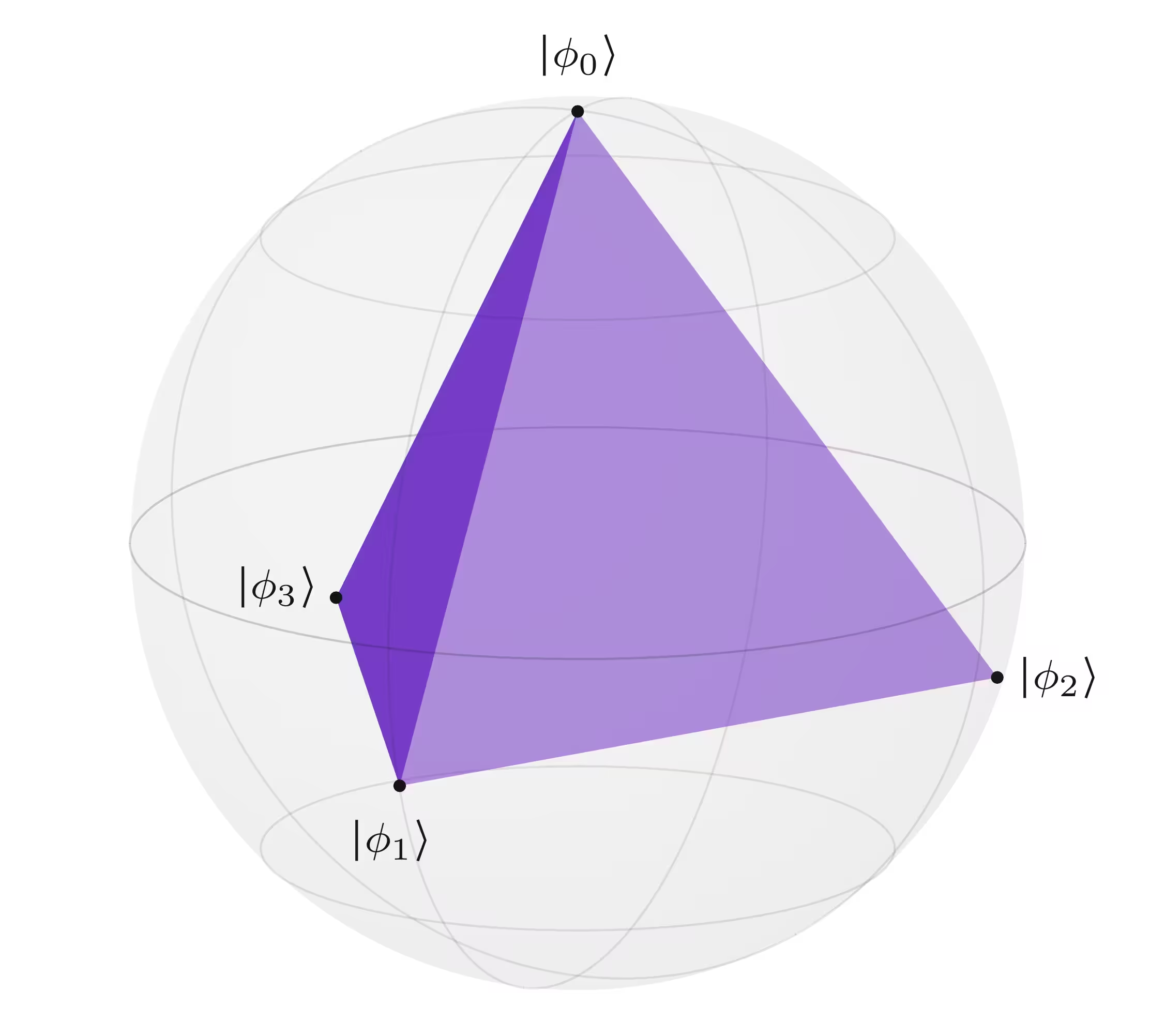
These four states are perfectly spread out on the Bloch sphere, each one equidistant from the other three and with the angles between any two of them always being the same.

Now let us define a measurement $\{P_0,P_1,P_2,P_3\}$ of a qubit by setting $P_a$ as follows for each $a=0,\ldots,3.$

$$P_a = \frac{\vert\phi_a\rangle\langle\phi_a\vert}{2}$$

We can verify that this is a valid measurement as follows.

1. Each $P_a$ is evidently positive semidefinite, being a pure state divided by one-half. That is, each one is a Hermitian matrix and has one eigenvalue equal to $1/2$ and all other eigenvalues zero.
2. The sum of these matrices is the identity matrix: $P_0 + P_1 + P_2 + P_3 = \mathbb{I}.$ The expressions of these matrices as linear combinations of Pauli matrices makes this straightforward to verify.

Measurements as channels

A second way to describe measurements in mathematical terms is as channels.

Classical information can be viewed as a special case of quantum information, insofar as we can identify probabilistic states with diagonal density matrices. So, in operational terms, we can think about measurements as being channels whose inputs are matrices describing states of whatever system is being measured and whose outputs are diagonal density matrices describing the resulting distribution of measurement outcomes.

We'll see shortly that any channel having this property can always be written in a simple, canonical form that ties directly to the description of measurements as collections of positive semidefinite matrices. Conversely, given an arbitrary measurement as a collection of matrices, there's always a valid channel having the diagonal output property that describes the given measurement as suggested in the previous paragraph. Putting these observations together, we find that the two descriptions of general measurements are equivalent.

Before proceeding further, let's be more precise about the measurement, how we're viewing it as a channel, and what assumptions we're making about it.

As before, we'll suppose that $\mathsf{X}$ is the system to be measured, and that the possible outcomes of the measurement are the integers $0,\ldots,m-1$ for some positive integer $m.$ We let $\mathsf{Y}$ be the system that stores measurement outcomes, so its classical state set is $\{0,\ldots,m-1\},$ and we represent the measurement as a channel named $\Phi$ from $\mathsf{X}$ to $\mathsf{Y}.$ Our assumption is that $\mathsf{Y}$ is classical — which is to say that no matter what state we start with for $\mathsf{X},$ the state of $\mathsf{Y}$ we obtain is represented by a diagonal density matrix.

We can express in mathematical terms that the output of $\Phi$ is always diagonal in the following way. First define the completely dephasing channel $\Delta_m$ on $\mathsf{Y}.$

$$\Delta_m(\sigma) = \sum_{a = 0}^{m-1} \langle a \vert \sigma \vert a\rangle \,\vert a\rangle\langle a\vert$$

This channel is analogous to the completely dephasing qubit channel $\Delta$ from the previous lesson. As a linear mapping, it zeros out all of the off-diagonal entries of an input matrix and leaves the diagonal alone.

And now, a simple way to express that a given density matrix $\sigma$ is diagonal is by the equation $\sigma = \Delta_m(\sigma).$ In words, zeroing out all of the off-diagonal entries of a density matrix has no effect if and only if the off-diagonal entries were all zero to begin with. The channel $\Phi$ therefore satisfies our assumption — that $\mathsf{Y}$ is classical — if and only if

$$\Phi(\rho) = \Delta_m(\Phi(\rho))$$

for every density matrix $\rho$ representing a state of $\mathsf{X}.$

Equivalence of the formulations

Channels to matrices

Suppose that we have a channel from $\mathsf{X}$ to $\mathsf{Y}$ with the property that

$$\Phi(\rho) = \Delta_m(\Phi(\rho))$$

for every density matrix $\rho.$ This may alternatively be expressed as follows.

$$\Phi(\rho) = \sum_{a = 0}^{m-1} \langle a \vert \Phi(\rho) \vert a\rangle\, \vert a\rangle\langle a \vert \tag{1}$$

Like all channels, we can express $\Phi$ in Kraus form for some way of choosing Kraus matrices $A_0,\ldots,A_{N-1}.$

$$\Phi(\rho) = \sum_{k = 0}^{N-1} A_k \rho A_k^{\dagger}$$

This provides us with an alternative expression for the diagonal entries of $\Phi(\rho)\!:$

$$\begin{aligned} \langle a \vert \Phi(\rho) \vert a\rangle & = \sum_{k = 0}^{N-1} \langle a \vert A_k \rho A_k^{\dagger} \vert a\rangle \\ & = \sum_{k = 0}^{N-1} \operatorname{Tr}\bigl( A_k^{\dagger} \vert a\rangle\langle a \vert A_k \rho\bigr)\\ & = \operatorname{Tr}\bigl(P_a\rho\bigr) \end{aligned}$$

for

$$P_a = \sum_{k = 0}^{N-1} A_k^{\dagger} \vert a\rangle\langle a \vert A_k.$$

Thus, for these same matrices $P_0,\ldots,P_{m-1}$ we can express the channel $\Phi$ as follows.

$$\Phi(\rho) = \sum_{a = 0}^{m-1} \operatorname{Tr}(P_a \rho) \vert a\rangle\langle a\vert$$

This expression is consistent with our description of general measurements in terms of matrices, as we see each measurement outcome appearing with probability $\operatorname{Tr}(P_a \rho).$

Now let's observe that the two properties required of the collection of matrices $\{P_0,\ldots,P_{m-1}\}$ to describe a general measurement are indeed satisfied. The first property is that they're all positive semidefinite matrices. One way to see this is to observe that, for every vector $\vert \psi\rangle$ having entries in correspondence with the classical state of $\mathsf{X}$ we have

$$\langle \psi \vert P_a \vert \psi\rangle = \sum_{k = 0}^{N-1} \langle \psi \vert A_k^{\dagger} \vert a\rangle\langle a \vert A_k\vert \psi\rangle = \sum_{k = 0}^{N-1} \bigl\vert\langle a \vert A_k\vert \psi\rangle\bigr\vert^2 \geq 0.$$

The second property is that if we sum these matrices we get the identity matrix.

$$\begin{aligned} \sum_{a = 0}^{m-1} P_a & = \sum_{a = 0}^{m-1} \sum_{k = 0}^{N-1} A_k^{\dagger} \vert a\rangle\langle a \vert A_k \\ & = \sum_{k = 0}^{N-1} A_k^{\dagger} \Biggl(\sum_{a = 0}^{m-1} \vert a\rangle\langle a \vert\Biggr) A_k \\ & = \sum_{k = 0}^{N-1} A_k^{\dagger} A_k \\ & = \mathbb{I}_{\mathsf{X}} \end{aligned}$$

The last equality follows from the fact that $\Phi$ is a channel, so its Kraus matrices must satisfy this condition.

Matrices to channels

Now let's verify that for any collection $\{P_0,\ldots,P_{m-1}\}$ of positive semidefinite matrices satisfying $P_0 + \cdots + P_{m-1} = \mathbb{I}_{\mathsf{X}},$ the mapping defined by

$$\Phi(\rho) = \sum_{a = 0}^{m-1} \operatorname{Tr}(P_a \rho) \vert a \rangle\langle a\vert$$

is indeed a valid channel from $\mathsf{X}$ to $\mathsf{Y}.$

One way to do this is to compute the Choi representation of this mapping.

$$\begin{aligned} J(\Phi) & = \sum_{b,c = 0}^{n-1} \vert b \rangle \langle c \vert \otimes \Phi(\vert b \rangle \langle c \vert)\\[1mm] & = \sum_{b,c = 0}^{n-1} \sum_{a = 0}^{m-1} \vert b \rangle \langle c \vert \otimes \operatorname{Tr}(P_a \vert b \rangle \langle c \vert) \vert a \rangle\langle a\vert\\[1mm] & = \sum_{b,c = 0}^{n-1} \sum_{a = 0}^{m-1} \vert b \rangle \langle b \vert P_a^T \vert c \rangle \langle c \vert \otimes \vert a \rangle\langle a\vert\\[1mm] & = \sum_{a = 0}^{m-1} P_a^T \otimes \vert a \rangle\langle a\vert \end{aligned}$$

The transpose of each $P_a$ is introduced for the third equality because

$$\langle c \vert P_a \vert b\rangle = \langle b \vert P_a^T \vert c\rangle.$$

This allows for the expressions $\vert b \rangle \langle b \vert$ and $\vert c \rangle \langle c \vert$ to appear, which simplify to the identity matrix upon summing over $b$ and $c,$ respectively.

By the assumption that $P_0,\ldots,P_{m-1}$ are positive semidefinite, so too are $P_0^{T},\ldots,P_{m-1}^{T}.$ In particular, transposing a Hermitian matrix results in another Hermitian matrix, and the eigenvalues of any square matrix and its transpose always agree. It follows that $J(\Phi)$ is positive semidefinite. Tracing out the output system $\mathsf{Y}$ (which is the system on the right) yields

$$\operatorname{Tr}_{\mathsf{Y}} (J(\Phi)) = \sum_{a = 0}^{m-1} P_a^T = \mathbb{I}_{\mathsf{X}}^T = \mathbb{I}_{\mathsf{X}},$$

and so we conclude that $\Phi$ is a channel.

Partial measurements

Suppose that we have multiple systems that are collectively in a quantum state, and a general measurement is performed on one of the systems. This results in one of the measurement outcomes, selected at random according to probabilities determined by the measurement and the state of the system prior to the measurement. The resulting state of the remaining systems will then, in general, depend on which measurement outcome was obtained.

Let's examine how this works for a pair of systems $(\mathsf{X},\mathsf{Z})$ when the system $\mathsf{X}$ is measured. (We're naming the system on the right $\mathsf{Z}$ because we'll take $\mathsf{Y}$ to be a system representing the classical output of the measurement when we view it as a channel.) We can then easily generalize to the situation in which the systems are swapped as well as to three or more systems.

Suppose the state of $(\mathsf{X},\mathsf{Z})$ prior to the measurement is described by a density matrix $\rho,$ which we can write as follows.

$$\rho = \sum_{b,c = 0}^{n-1} \vert b\rangle\langle c\vert \otimes \rho_{b,c}$$

In this expression we're assuming the classical states of $\mathsf{X}$ are $0,\ldots,n-1.$

We'll assume that the measurement itself is described by the collection of matrices $\{P_0,\ldots,P_{m-1}\}.$ This measurement may alternatively be described as a channel $\Phi$ from $\mathsf{X}$ to $\mathsf{Y},$ where $\mathsf{Y}$ is a new system having classical state set $\{0,\ldots,m-1\}.$ Specifically, the action of this channel can be expressed as follows.

$$\Phi(\xi) = \sum_{a = 0}^{m-1} \operatorname{Tr}(P_a \xi)\, \vert a \rangle \langle a \vert$$

Outcome probabilities

We're considering a measurement of the system $\mathsf{X},$ so the probabilities with which different measurement outcomes are obtained can depend only on $\rho_{\mathsf{X}},$ the reduced state of $\mathsf{X}.$ In particular, the probability for each outcome $a\in\{0,\ldots,m-1\}$ to appear can be expressed in three equivalent ways.

$$\operatorname{Tr}\bigl( P_a \rho_{\mathsf{X}}\bigr) = \operatorname{Tr}\bigl( P_a \operatorname{Tr}_{\mathsf{Z}}(\rho)\bigr) = \operatorname{Tr}\bigl( (P_a \otimes \mathbb{I}_{\mathsf{Z}}) \rho \bigr)$$

The first expression naturally represents the probability to obtain the outcome $a$ based on what we already know about measurements of a single system. To get the second expression we're simply using the definition $\rho_{\mathsf{X}} = \operatorname{Tr}_{\mathsf{Z}}(\rho).$

To get the third expression requires more thought — and learners are encouraged to convince themselves that it is true. Here's a hint: The equivalence between the second and third expressions does not depend on $\rho$ being a density matrix or on each $P_a$ being positive semidefinite. Try showing it first for tensor products of the form $\rho = M\otimes N$ and then conclude that it must be true in general by linearity.

While the equivalence of the first and third expressions in the previous equation may not be immediate, it does make sense. Starting from a measurement on $\mathsf{X},$ we're effectively defining a measurement of $(\mathsf{X},\mathsf{Z}),$ where we simply throw away $\mathsf{Z}$ and measure $\mathsf{X}.$ Like all measurements, this new measurement can be described by a collection of matrices, and it's not surprising that this measurement is described by the collection

$$\{P_0\otimes\mathbb{I}_{\mathsf{Z}}, \ldots, P_{m-1}\otimes\mathbb{I}_{\mathsf{Z}}\}.$$

States conditioned on measurement outcomes

If we want to determine not only the probabilities for the different outcomes but also the resulting state of $\mathsf{Z}$ conditioned on each measurement outcome, we can look to the channel description of the measurement. In particular, let's examine the state we get when we apply $\Phi$ to $\mathsf{X}$ and do nothing to $\mathsf{Z}.$

$$\begin{aligned} (\Phi\otimes\operatorname{Id}_{\mathsf{Z}})(\rho) & = \sum_{b,c = 0}^{n-1} \Phi(\vert b\rangle\langle c\vert) \otimes \rho_{b,c}\\ & = \sum_{a = 0}^{m-1} \sum_{b,c = 0}^{n-1} \operatorname{Tr}(P_a \vert b\rangle\langle c\vert) \,\vert a\rangle \langle a \vert \otimes \rho_{b,c}\\ & = \sum_{a = 0}^{m-1} \vert a\rangle \langle a \vert \otimes \sum_{b,c = 0}^{n-1} \operatorname{Tr}(P_a \vert b\rangle\langle c\vert) \rho_{b,c}\\ & = \sum_{a = 0}^{m-1} \vert a\rangle \langle a \vert \otimes \sum_{b,c = 0}^{n-1} \operatorname{Tr}_{\mathsf{X}}\bigl((P_a\otimes\mathbb{I}_{\mathsf{Z}}) (\vert b\rangle\langle c\vert\otimes\rho_{b,c})\bigr)\\ & = \sum_{a = 0}^{m-1} \vert a\rangle \langle a \vert \otimes \operatorname{Tr}_{\mathsf{X}}\bigl((P_a \otimes \mathbb{I}_{\mathsf{Z}}) \rho\bigr) \end{aligned}$$

Note that this is a density matrix by virtue of the fact that $\Phi$ is a channel, so each matrix $\operatorname{Tr}_{\mathsf{X}}\bigl((P_a \otimes \mathbb{I}_{\mathsf{Z}}) \rho)$ is necessarily positive semidefinite.

One final step transforms this expression into one that reveals what we're looking for.

$$\sum_{a = 0}^{m-1} \operatorname{Tr}\bigl((P_a \otimes \mathbb{I}_{\mathsf{Z}}) \rho)\, \vert a\rangle \langle a \vert \otimes \frac{\operatorname{Tr}_{\mathsf{X}}\bigl((P_a \otimes \mathbb{I}_{\mathsf{Z}}) \rho)}{\operatorname{Tr}\bigl((P_a \otimes \mathbb{I}_{\mathsf{Z}}) \rho)}$$

This is an example of a classical-quantum state,

$$\sum_{a = 0}^{m-1} p(a)\, \vert a\rangle\langle a\vert \otimes \sigma_a,$$

like we saw in the Density matrices lesson. For each measurement outcome $a\in\{0,\ldots,m-1\},$ we have with probability

$$p(a) = \operatorname{Tr}\bigl((P_a \otimes \mathbb{I}_{\mathsf{Z}}) \rho)$$

that $\mathsf{Y}$ is in the classical state $\vert a \rangle \langle a \vert$ and $\mathsf{Z}$ is in the state

$$\sigma_a = \frac{\operatorname{Tr}_{\mathsf{X}}\bigl((P_a \otimes \mathbb{I}_{\mathsf{Z}}) \rho)}{\operatorname{Tr}\bigl((P_a \otimes \mathbb{I}_{\mathsf{Z}}) \rho)}. \tag{2}$$

That is, this is the density matrix we obtain by normalizing

$$\operatorname{Tr}_{\mathsf{X}}\bigl((P_a \otimes \mathbb{I}_{\mathsf{Z}}) \rho)$$

by dividing it by its trace. (Formally speaking, the state $\sigma_a$ is only defined when the probability $p(a)$ is nonzero; when $p(a) = 0$ this state is irrelevant, for it refers to a discrete event that occurs with probability zero.)

Naturally, the outcome probabilities are consistent with our previous observations.

In summary, this is what happens when the measurement $\{P_0,\ldots,P_{m-1}\}$ is performed on $\mathsf{X}$ when $(\mathsf{X},\mathsf{Z})$ is in the state $\rho.$

1. Each outcome $a$ appears with probability $p(a) = \operatorname{Tr}\bigl((P_a \otimes \mathbb{I}_{\mathsf{Z}}) \rho).$
2. Conditioned on obtaining the outcome $a,$ the state of $\mathsf{Z}$ is then represented by the density matrix $\sigma_a$ shown in the equation $(2),$ which is obtained by normalizing $\operatorname{Tr}_{\mathsf{X}}\bigl((P_a \otimes \mathbb{I}_{\mathsf{Z}}) \rho).$

Generalization

We can adapt this description to other situations, such as when the ordering of the systems is reversed or when there are three or more systems. Conceptually it is straightforward, although it can become cumbersome to write down the formulas.

In general, if we have $r$ systems $\mathsf{X}_1,\ldots,\mathsf{X}_r,$ the state of the compound system $(\mathsf{X}_1,\ldots,\mathsf{X}_r)$ is $\rho,$ and the measurement $\{P_0,\ldots,P_{m-1}\}$ is performed on $\mathsf{X}_k$, the following happens.

1. Each outcome $a$ appears with probability

   $$p(a) = \operatorname{Tr}\bigl((\mathbb{I}_{\mathsf{X}_1}\otimes \cdots \otimes\mathbb{I}_{\mathsf{X}_{k-1}} \otimes P_a \otimes \mathbb{I}_{\mathsf{X}_{k+1}} \otimes \cdots \otimes\mathbb{I}_{\mathsf{X}_r}) \rho\bigr).$$

2. Conditioned on obtaining the outcome $a,$ the state of $(\mathsf{X}_1,\ldots,\mathsf{X}_{k-1},\mathsf{X}_{k+1},\ldots,\mathsf{X}_r)$ is then represented by the following density matrix.

   $$\frac{\operatorname{Tr}_{\mathsf{X}_k}\bigl((\mathbb{I}_{\mathsf{X}_1}\otimes \cdots \otimes\mathbb{I}_{\mathsf{X}_{k-1}} \otimes P_a \otimes \mathbb{I}_{\mathsf{X}_{k+1}} \otimes \cdots \otimes\mathbb{I}_{\mathsf{X}_r}) \rho\bigr)}{\operatorname{Tr}\bigl((\mathbb{I}_{\mathsf{X}_1}\otimes \cdots \otimes\mathbb{I}_{\mathsf{X}_{k-1}} \otimes P_a \otimes \mathbb{I}_{\mathsf{X}_{k+1}} \otimes \cdots \otimes\mathbb{I}_{\mathsf{X}_r}) \rho\bigr)}$$